AtCoder Grand Contest 033

AtCoder Grand Contest 033

Source codes

• My submissions (AtCoder)
• My source codes (GitHub)

Solutions

A - Darker and Darker

普通に BFS をすればよろしい。

B - LRUD Game

$0$-indexed とする。操作を逆順に見ていく。時系列を逆順にする。

定義： 領域 $D$ がその時の 安全な領域 であるとは、任意の点 $p \in D$ に対し、任意の高橋君の操作に対し、青木君の操作が存在し、その点にある駒が落ちないようにゲームを終了でき、任意の $p \not \in D$ に対してはそうでないことを指す。

初期状態は $D = H \times W = [0, H - 1] \times [0, W - 1]$ である。

青木君の方は、 $D$ を拡張することができる。例えば 'L' が来ると、 $D$ の右側のマスを $+1$ しても大丈夫なことがわかる。そのような駒があったとしたら、青木君はその 'L' で左に戻せばそれまでの安全な領域に駒を動かすことができるからだ。ただし全領域からははみ出さないようにする必要がある。

高橋君の方は、 $D$ を狭めることができる。例えば 'L' が来ると、 $D$ の左側のマスを $-1$ することがわかる。そのような駒があったとしたら、高橋君はその 'L' で左に動かせばそれまでの安全な領域の外に駒を動かすことができるからだ。

以上の操作と初期状態を踏まえれば、常に $D = [up, down] \times [left, right]$ の形をしている。愚直にシミュレーションできる。答えが "YES" であるための必要十分条件は常に $D \neq \emptyset$ であること、かつ、最終局面で $(s_c, s_r) \in D$ であることである。

ポイント

嘘解法が通されたらしい。

C - Removing Coins

解答

木の直径を $L$ とすると、 $L \% 3 = 1$ のとき "Second", そうでないとき "First" である。

解答の正当化

操作によってコインが置かれなかった頂点は、木から取り除くものとして良い。するとこの操作は、

• 最初に選ぶ頂点が根である場合：その根以外の根を $1$ 段階取り除く
• 最初に選ぶ頂点が根以外である場合：全ての根を $1$ 段階取り除く

ことに相当する。

命題 1：木の直径 $L$ は、 1 回の操作により、 $L - 1$ または $L - 2$ になる。ただし悲負の数を考えるものとする。

証明：木の直径を構成する任意の頂点を指定して操作すると、直径は $L - 1$ になる。そうでなければ $L - 2$ になる。

命題 2：木の直径を $L$ とする。このとき Grundy 数 $G$ は、以下で与えられる。 \[ G = G(L) = \begin{cases} 0 & L \% 3 = 1, \\
1 & L \% 3 = 0, \\
2 & L \% 3 = 3. \end{cases} \] すなわち、 $1, 0, 2, 1, 0, 2, \dots$ となる。

証明： $L$ についての数学的帰納法による。 $L = 0$ のとき、どのように操作しても木は $\emptyset$ になるので、後手は負ける。よって Grundy 数は $1$ である。 $L = 1$ のとき、操作により $L = 0$ の木にしかならないので、 Grundy 数は $0$ である。 $L \geq 2$ とし、 $L - 1$, $L - 2$ での成立を仮定する。このとき、操作により直径が $L - 1$ の木、または、直径が $L - 2$ の木にしかならない。よって Grundy 数の定義により、次式が成立する。 \[ G = \min \{ n \in \mathbb{N} \mid n \neq G(L - 1) \land n \neq G(L - 2) \}. \] 帰納法の仮定に基づき場合分けをすることにより、命題 2 が示される。

木の直径 $L$ は DFS を 2 回することにより $O(N)$ で求まる。 $L \% 3 = 1$ のとき、答えは "Second" であり、そうでなければ "First" である。

ポイント

直径に気づけば、解けたと思う。もう少し大きい例で試してみるべきだった。

D - Complexity

Let $N = \max(H, W)$. Assume $0$-indexed.

Observation

This problem has a strict memory limit. To be short, we have to solve this problem in less than or equal to $O(N ^ 3 \log N)$-time.

First we notice that, suppose we have two rectangles $R _ 0$ and $R _ 1$ with $R _ 0 \subset R _ 1$, the complexity of $R _ 0$ is less than or equal to that of $R _ 1$.

Second we notice that in this problem the complexity of the entire grid does not exceed $16$. This is where $\log N$ appears.

Thus, we define two DP tables as follows.

$dp1[k][x _ 0][x _ 1][y _ 0] = y _ 1$: Fix the level $k$ and the $x$-range $[x _ 0, x _ 1)$. It gives the maximum of $y _ 1$ that satisfies the level $[x _ 0, x _ 1) \times [y _ 0, y _ 1)$ is less than or equal to $k$.
$dp2[k][y _ 0][y _ 1][x _ 0] = x _ 1$: Fix the level $k$ and the $y$-range $[y _ 0, y _ 1)$. It gives the maximum of $x _ 1$ that satisfies the level $[x _ 0, x _ 1) \times [y _ 0, y _ 1)$ is less than or equal to $k$.

We can update $dp1$ and $dp2$ by doubling.

Solution

First of all we have calculate $dp1[0]$ and $dp2[0]$ directly from the input. This is a routine work, but take care not to make a bug.

Then, we update $dp1[k]$ and $dp2[k]$ by using both $dp1[k - 1]$ and $dp2[k - 1]$ for $k = 1, \dots, 16$.

Idea

By definition, we admit that the complexity of the rectangle $R$ is less than or equal to $k$ if and only if there exists a separation $R _ 1 \cup R _ 2 = R$ whose complexity is both less than or equal to $k - 1$. If the line of the separation is parallel to $x$-axis, we can extract the information from $dp1$. If it is parallel to $y$-axis, we can from $dp2$. This is done by the combination of two-pointer and doubling.

Algorithm

For $k = 1, \dots, 16$, for $0 \leq x _ 0 \leq x _ 1 \leq H$, we compute $dp1[k][x _ 0][x _ 1]$. Let $y _ 0 = y _ 1 = W$. While $y _ 0 \geq 0$, if either of the followings holds; \[ \begin{align} dp1[k - 1][x _ 0][x _ 1][dp1[k - 1][x _ 0][x _ 1][y _ 0]] &\geq y _ 1, \\
dp2[k - 1][y _ 0][y _ 1][dp2[k - 1][y _ 0][y _ 1][x _ 0]] &\geq x _ 1, \end{align} \] we set $dp1[k][x _ 0][x _ 1][y _ 0] = y _ 1$ and $y _ 0 \mathbin{ {-} {-} };$; otherwise $y _ 1 \mathbin{ {-} {-} }$. We can also fill $dp2[k]$ in the same way.

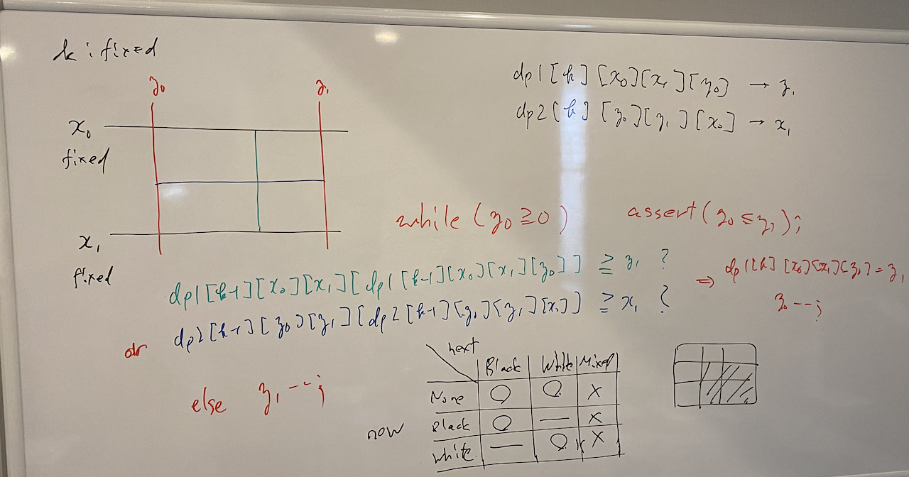
The answer is \[ \text{argmin} _ {k} dp0[k][0][H][0] = W. \]

E - Go around a Circle

Observation

Without loss of generalities, we assume that $S$ starts by R. If we have BB on the circle grid, we see that this is invalid. Therefore, each B must be alone.

We separate into two cases.

Case 1: $S$ consists of only Rs

In this case, we have no other restriction.

Case 2: $S$ contains a B

We first claim that each length of continuous Rs on the grid must be odd. Assume to the contrary that there exist the continuous Rs whose length is even. Let $L$ be the length of the first continuous Rs. If $L$ is even, we starts at the point adjacent to the edge between these Rs and B to see that the generation is impossible. If $L$ is odd, we starts at the edge between these Rs and B to see the same result.

Furthermore, we have the upper bound of the length of each segment of R.

• The first segment of R
  • Starts at any point. Ends at one of the edge points between R and B.
  • If $L$ is even, the upper bound is $L + 1$. If $L$ is odd, the upper bound is $L$.
• The inner segments of R
  • Starts and ends at one of the edge points between R.
  • If $L$ is even, it does not restrict the upper bound. If $L$ is odd, the upper bound is $L$.
• The last segment of R
  • Starts at one of the edge points between R and B. Ends at any point.
  • This does not restrict the upper bound.

Therefore, we have a upper bound $X = max\_length(S)$.

On the contrary, if the grid satisfies all the conditions describe above, we see that we can generate $S$ from every point on the grid.

In addition, it follows that $N$ must be even since the number of segment of Rs and that of segment of Bs (actually it is alone) are the same and each length of them are all odd.

Case 1: DP Part

First, we solve the problem on the line.

Definition

$dp[i][j] = $ the number of possibilities to color out the segment $[0, i - 1)$, where the last segment has $j$ Bs.

Initial State

$dp[0][0] = 1$; otherwise $0$.

Transition

For $i = 1, \dots, N$, we execute \[ \begin{align} dp[i][0] &= dp[i - 1][0] + dp[i - 1][1], \\
dp[i][1] &= dp[i - 1][0]. \end{align} \]

Solution for Original Problem

The original problem is about the circle grid. We have to care for both side of edges. There is three possibilities.

1. Starts and ends by R,
2. Starts by R and ends by B,
3. Starts by B and ends by R.

How many possibilities are there when we fill the inner part? For the first case, it is $dp[N - 2][0] + dp[N - 2][1]$. For the second and third cases, it is $dp[N - 2][0]$. Therefore the answer is \[ 3 dp[N - 2][0] + dp[N - 2][1]. \]

Case 2: DP Part

Before we argue the implement, we summarize the conditions.

• Each B must be alone.
• The length of each segment of Rs must be odd and less than or equal to $X$.

As we pointed out before, $N$ must be even. We come up with a good idea. For either odd or even $i$, all the $i$-th color will be R. Thus we consider the $N / 2$-color grid. The answer will be doubled. Hereinafter we set $N \gets N / 2$ and $X \gets X / 2$. Then, the condition will be transformed as follows.

• (There remains nothing for B.)
• The length of each segment of Rs must be less than or equal to $X$.

As we demonstrated just before, we solve the problem on the line and go to further results.

Definition

$dp[i][j] = $ the number of possibilities to color out the segment $[0, i - 1)$, where the last segment has $j$ Rs.

The space complexity will be $O(N ^ 2)$. Thus we will have to fasten the manipulation later.

Initial State

$dp[0][0] = 1$, otherwise $0$.

Transition

On this DP, some speeding up will be needed later. Thus we think of the collecting DP instead of the gathering DP.

For $i = 1, \dots, N$, we execute the following. \[ \begin{align} dp[i][0] &= \sum _ {j = 0} ^ {X} dp[i - 1][j], \\
dp[i][j] &= dp[i - 1][j - 1] \text{ for } j = 1, \dots X. \end{align} \]

Convert $dp$ into $DP$

What we need is \[ DP[i] = \sum _ {j = 0} ^ X dp[i][j]. \]

We want to speed up the transition part. Fortunately, this is done r ather easily. \[ \begin{align} DP[i] &= dp[i][0] + \sum _ {j = 1} ^ X dp[i][j] \\
&= \sum _ {j = 0} ^ X dp[i - 1][j] + \sum _ {j = 1} ^ X dp[i - 1][j - 1] \\
&= 2DP[i - 1] - dp[i - 1][X] \\
&= \begin{cases} 2DP[i - 1] - dp[i - 1 - X][0] & i - 1 - X \geq 0, \\
2DP[i - 1] & \text{otherwise}. \end{cases} \\
&= \begin{cases} 2DP[i - 1] - DP[i - 2 - X] & i - 1 - X > 0, \\
2DP[i - 1] - 1 & i - 1 - X = 0, \\
2DP[i - 1] & \text{otherwise}. \end{cases} \end{align} \]

Be careful for the last manipulation! $dp[i - 1 - X][0] = DP[i - 2 - X]$ follows when $i - 1 - X > 0$.

Solution for Original Problem

To calculate the circle grid version, we have to count the length between the first and the last Bs on the segment. But we can overcome this hardness by fixing the places of the first and the last Bs.

Suppose that the length of the circle-continuous last and first Rs is $K$. The possibilities of the places of the first and last B will be $(K + 1)$. The inner part will be filled as we have argued above. Then, the answer is roughly as follows. \[ \sum _ {K = 0} ^ X (K + 1)DP[N - K - 2]. \]

We promise two rules. First, the out-of-range will be $0$ of course. Second, we have to consider the case that the first B and the last B are the very same. In this case, there is one B and others are all R. The number of the possibilities is $N$.

F - Adding Edges

Overview

This problem can be solved by considering the following two steps.

1. Re-generate an equivalent graph $G$ that flushes the same answer but easy to count.
2. Count the number of edges in $O(N ^ 2)$-time.

Technically speaking, Step 1 is difficult. In terms of the hardness of coming up with the idea, Step 2 is rather difficult.

Convert $G$ into an equivalent graph, then count

Let $a$, $b$ and $c$ be vertexes on a same path in this order. Since, finally, we add the edges that generate the triangles, we can say that the following states are equivalent.

• Edge $(a, b)$ and $(b, c)$
• Edge $(a, c)$ and $(b, c)$
• Edge $(a, b)$ and $(a, c)$
• Edge $(a, b)$, $(b, c)$ and $(c, a)$

Suppose that $G$ has only the first type of the edges. Then, we can count the number of edges on the final state by DFS from each vertex, which runs in $O(N ^ 2)$-time. In addition, we can accept the forth type.

How does the fact that $G$ has only the first and forth type of the edges make it easy to calculate the answer? In this case, all the edges are “flat”. More precisely, we don’t have to care for returning-back type adding-edge manipulations. Therefore, we can use DFS.

Example

To consider how to possess $G$ and implement the algorithm later, we look at it carefully by using examples. Let’s consider the sample input 1. Assume that we can flatten $G$ described as the following picture.

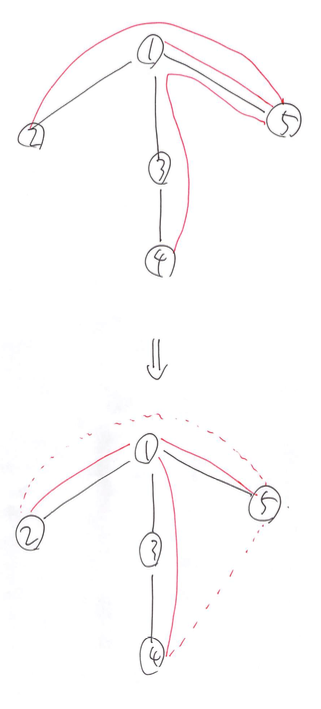
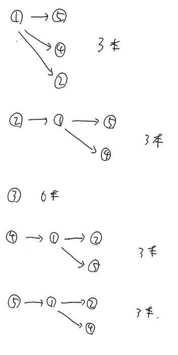
Then, we can count the answer as follows.

What we want to point out here is that, for example, we count the edge $(2, 5)$ by counting the edge $(1, 5)$ instead of that. This tells us how to possess $G$ and build the algorithm. First, it will be good that we have $G$ by adjacent matrix. Second, we use DFS by remembering not only its parent but also its root. This enable us to consider $(2, 5)$ by $(1, 5)$.

How to generate an equivalent $G$

We can keep $T$ by its adjacent list in a normal way. As we discussed before, however, we possess the state of $G$ by vector<vector<int>> G;. The formal definition is as follows.

$G[v][w] = w$ if there exists an edge $(v, w)$ in $G$; one of the inner vertexes which is connected to either $v$ or $w$; empty otherwise.

Here we promise that the condition that $(v, w)$ exists is equivalent to $G[v][w] = w$.

We generate $G$ with the triangles “flat” as we discussed above. There are two types of situations we have to care for. Suppose that the vertexes $a$, $b$ and $c$ are on a same path in this order.

• When we add $(a, b)$, we have to find all $c$ with $(a, c)$ and execute $(b, c)$.
• When we add $(a, c)$, we have to find all $b$ with either $(a, b)$ or $(b, c)$ exists and we execute the other.

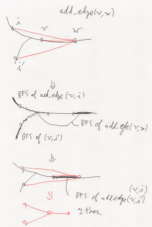
Our algorithm to generate $G$ is as follows.

1. We execute void add_edge(int v, int w); for all the queries.
2. In add_edge, the main idea is to add edge $(v, w)$ to $G$ and calculate $G[v][i]$ and $G[w][i]$ for the outside of $(v, w)$. This is done by BFS.
   • We set $G[w][i] = G[i][w] = v$ if it is empty and continue BFS.
   • If it is an edge, i.e., $G[w][i] = i$, we call add_edge(v, i);. Since there exist two edges $(w, i)$ and $(w, v)$, we have to add $(v, i)$ for our rule. We stop the BFS.
   • Otherwise, we just stop the BFS.
3. In this recursion, we have to fix some states. If $G[v][w] = w$ and/or $G[w][v] = v$, we have no operation. If $G[v][w] = e$ for some other vertex, it means that we have to execute both add_edge(G[v][w], w); and add_edge(G[v][w], v); instead of the original one. Here, we note that actually we execute either of the two, not both.

Time complexity

We want to estimate the time complexity of the algorithm above. The following lemma is a key.

Lemma F.1: Take a moment in executing this algorithm. Let $A$ be the number of manipulations we have done. Let $B$ is the sum of the length of the paths on $G$. Here, we count the path which is not considered yet as $N - 1$ of its length. Then, the following equation follows. \[ A + B \leq MN + o(NM). \]

Proof: At the very first time, $A = 0$ and $B = M(N - 1)$ by definition. We consider each steps. Assume that we add $(v, w)$ to $G$. If the fixed points works, the manipulation is $0$ or less than the the argument below. Hence we consider the original query. Let $L$ the number of edges included between $v$ and $w$. By BFS, we fill the outside of $(v, w)$. Thus the number of manipulation is no more than $2 + (N - 1 - L)$. Before stopping BFS, we have additional tasks add_edge(v, i);; others are ignorable. In addition, its new BFS from $i$ to the outer side is ignorable since the number of the actual manipulation is included in the previous estimate $2 + (N - 1 - L)$. To the contrary, its new BFS from $v$ to the inner side continues until it reaches, for example, $w$. The fact is that the number of the manipulation needed is equal to the overlapping length. This does not exceed $L$ and the remain will be used by the same argument in the future, or won’t be reduced. This fact is complicated to prove, since we have to separate the deep recursion. But we can see the example on the picture below.

By Lemma F.1, we see that our algorithm works in $O(NM)$-time.

Others